Monolithic Unfitted Space-Time FEM for an Osmotic Cell Swelling Problem
1. Scope of the thesis
Let \(u\) be the concentration of a dissolved species in an osmotic cell and \(\mu\) be a corresponding (constant) diffusion coefficient. A standard linear diffusion law is assumed to describe the distribution of \(u\) inside \(\Omega\). On the boundary of the domain we demand conservation of mass which results in the boundary conditions which state that the diffusive flux at the boundary \(-\mu \nabla u \cdot n_{\partial \Omega}\) coincides with the convective flux due to the motion of the boundary \(u \mathcal{V}_n\) with \(\mathcal{V}_n\) the velocity of the boundary in normal direction. Finally, we note that the evolution of the cell is determined by the normal velocity \(\mathcal{V}_n\) of the surface. The surface tension force is modeled with \(-\alpha \kappa\), where \(\kappa\) is the mean curvature of the surface and \(\alpha\) is a positive constant and the counteracting osmotic pressure is simply modeled as \(\beta u\) with a positive constant \(\beta\). Here, \(\kappa\) is the mean curvature with \(\kappa > 0\) for the boundary of convex domains. The set of equations is
\begin{align} \partial_t u - \mathrm{div} (\mu \nabla u) = & \, f && ~~\text{in}~~ \Omega(t), & t \in (0,T],\\ u \mathcal{V}_n + \mu \nabla u \cdot n_{\partial \Omega} = & \, 0 && ~~\text{on}~~ \partial \Omega(t), & t \in (0,T],\\ -\alpha \kappa + \beta u = & \, \mathcal{V}_n && ~~\text{on}~~ \partial \Omega(t), & t \in (0,T]. \end{align}
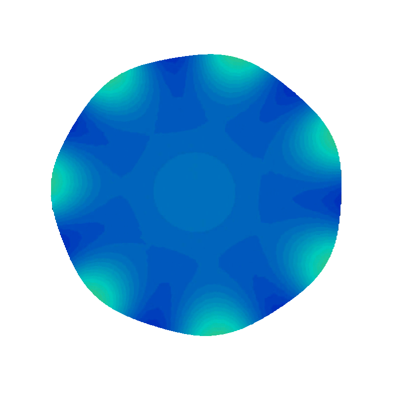
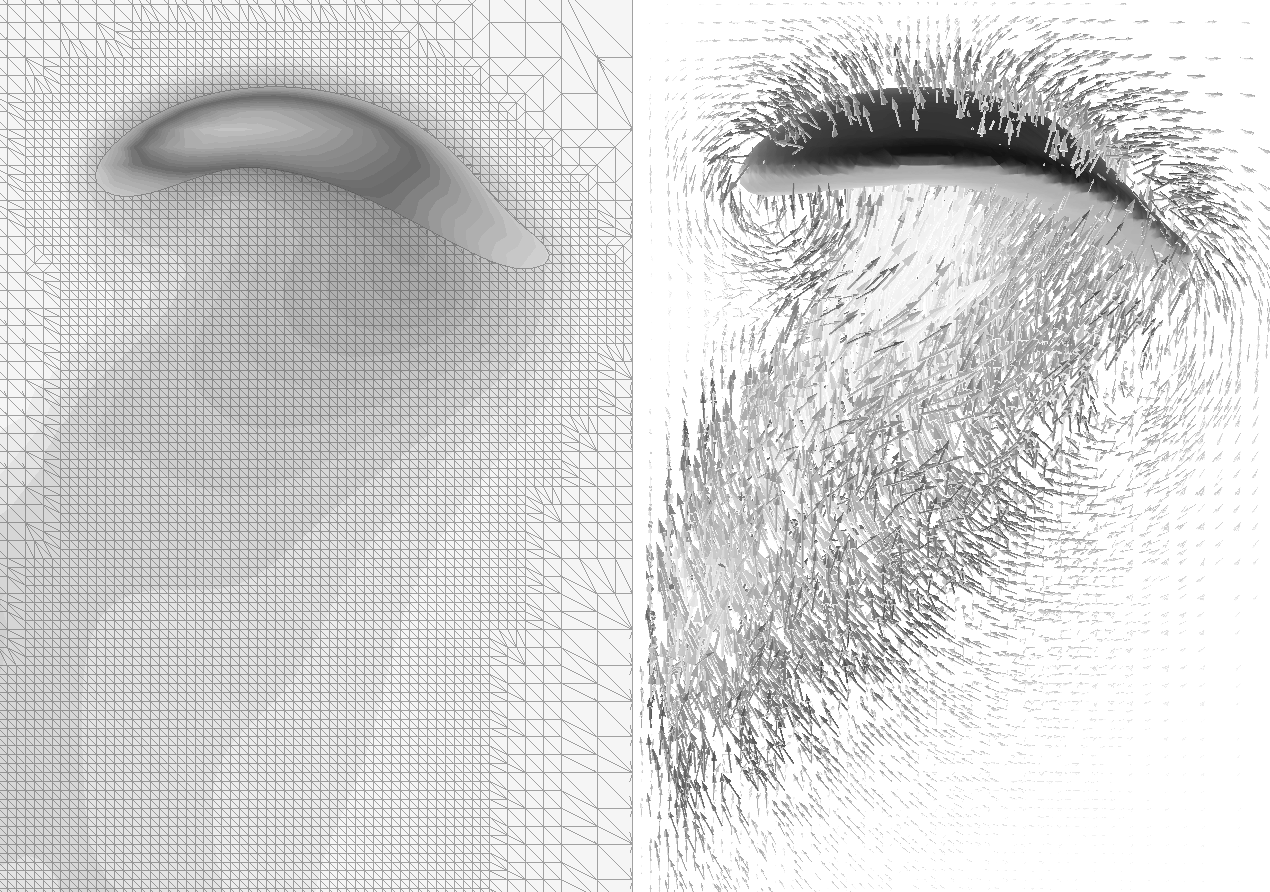
An examplary evolution of the geometry and the concentration field is depicted here (cf. also this video):


Several extensions to the model are possible to involve more complex behavior, for instance by considering PDEs also outside or on the surface or involving also balance equations for the momentum, cf. [2] [3]. In this project we want to focus on this simple model problem which already contains sufficient complexity to address the most important challenges for numerical discretizations. This problem has also been considered in [1] using diffuse interface models.
For the discretization we consider an unfitted setting where the geometry is described through a level set function, i.e. \(\Omega(t) = \{ \phi(t) < 0 \}\) for a scalar function on a typically simple domain \(\widetilde{\Omega}\).
The problem consists of essentially two subproblems:
- the evolution of the concentration field and
- the evolution of the level set function.
For the latter there are two different approaches. Depending on the approach the second problem may also be split into the determination of a velocity field and the evolution of the level set function. Furthermore, the subproblems are strongly coupled, i.e. the level set evolution influences the concentration field through the domain boundary. The concentration field (and the geometry itself) influence the level set evolution. For the subproblems there exists preliminary work (theoretical and implementation). For some problems to a larger, for others to a smaller extend.
In this thesis we aim at discretizing the problem in a time stepping manner. However, in every time step we want to solve all three subproblems in a space-time formulation which we strongly couple with a fixed point iteration yielding a monolithic space-time solver.
The primary goal of the thesis is the development of a fully working numerical solver. The topic however offers many open directions. Especially the nonlinear coupling of space-time unknowns is rather unusual, especially in an unfitted setting. One of many interesting questions is under which conditions the fix point iteration converges (theoretically and/or practically). Another one is how the convergence speed can be accelerated. Initially, we would consider piecewise linear functions in space (and time) only, but would like to extend this to higher order discretizations in space and time as well.
The topic heavily builds on the previous works in the Master's theses [6] [7].
2. Discretization spaces and general approach
Velocity field, level set function and concentration will be discretized by space-time finite elements. To describe more details we need some notation:
Let \(V_h\) be a scalar finite element space of continuous piecewise polynomials on \(\widetilde{\Omega}\) and \(W_h = V_h \otimes \mathcal{P}^k(t_{n-1},t_n)\) a corresponding space-time finite element space.
The notation \({\cdot}_n\) indicates a space-time functions in the interval \(I_n := (t_{n-1},t_n)\). The superscript index \(k\) is used for iteration index within the fixed point iteration in one time step whereas the subscript \(n\) is used to indicate the time interval or time step. \(\hat{\cdot}_n\) indicates a purely spatial function at \(t_n\), typically the (upper) limit from the time interval \(I_{n-1}\) or initial data.
The involved functions are in the following finite element spaces: level set function \(\phi_n^k \in W_{h}\) (hence \(\hat{\phi}_{n-1} \in V_{h}\)), concentration field \(u_n^k \in W_{h}\) (hence \(\hat{u}_{n-1} \in V_{h}\)).
3. Time loop
3.1. Initialization
Initial values \(\hat{\phi}_{0}\), \(\hat{u}_{0}\) are needed.
3.2. Iteration within one time step
The geometrically nonlinear problem is solved by a fixed point iteration. After initialization with \(\phi_n^0 = \hat{\phi}_{n-1} \otimes 1\), i.e. constant domain in the current time step, the following steps are iterated until convergence.
3.2.1. Unfitted space-time discretization of the concentration field
[\(u_n^{k+1} \leftarrow (\phi_n^k,\hat{u}_{n-1})\)]
An unfitted space-time formulation for a time step from \(t_{n-1}\) to \(t_n\) with given initial data \(\hat{u}(t_{n-1})\) takes the form: \begin{align} & - \int_{Q^n} u \frac{\partial v}{\partial t} \, dx + \int_{Q^n} \mu \nabla u \nabla v \, dx + \int_{\Omega(t_n)} u(t_n) v(t_n) \, dx + j_h^n(u,u) \\ &= \int_{\Omega(t_{n-1})} \hat{u}(t_{n-1}) v(t_{n-1}) \, dx,~ \forall v \in V_h^n \end{align} where \(V_h^n=\mathcal{R}^n V_h\) is the fictitious domain space-time finite element space with the standard tensor product finite element space \(V_h\) which is defined a priori w.r.t. the background mesh and the restriction operator \(\mathcal{R}^n\) corresponding to the space-time domain of the time step (hence depending on \(\phi^k\)). \(j_h\) is a stabilization bilinear form (``ghost penalty'').
3.2.2A. Evolution of the interface, Approach A:
The evolution of the domain is captured by the level set function \(\phi_n^k\). A suitable model for the evolution of the level set equation is \begin{align} \label{eq:osm:lseta} \tag{L} \frac{\partial_t \phi_n^k}{\Vert \nabla \phi_n^k \Vert} - \alpha \ \mathrm{div} \left( \frac{\nabla \phi_n^k}{\Vert \nabla \phi_n^k \Vert} \right) + \beta U_n^k = 0, \end{align} which has been considered in [7]. This is a modified version of the well-known mean curvature flow problem, cf. [5]. Here, \(\tilde{\Omega}\) is the fictitious domain which is defined by the background mesh which is used in the discretization and \(U_n^k\) is a suitable smooth extension of the quantity \(u_n^k\) which is originally only defined on \(\Omega(t)\). For the discretization of \eqref{eq:osm:lseta} a standard space-time finite element method combined with a method of lines can be applied. In order to do this step the extension \(U_n^k = \mathcal{E}_\Omega u_n^k\) needs to be constructed.
3.2.2A.1. Extension of the concentration field
[\(U_n^{k} \leftarrow u_n^k\)]
We use a ``ghost penalty'' extension mechanism, see [7] and [8].
3.2.2A.2. Solution of the parabolic level set evolution equation
[\(\phi_n^{k} \leftarrow (U_n^k,\hat{\phi}_{n-1}^k)\)]
Solve \eqref{eq:osm:lseta} in a space-time formulation.
3.2.2B. Evolution of the interface, Approach B:
3.2.2B.1.
t.b.d.3.3. Possible re-initialization
\(\phi_n' = R(\phi_n)\) where \(R\) should approximately keep the zero-level while enforcing an (almost) signed distance property \(\Vert \nabla \phi \Vert_2 \simeq 1\) (pointwise). This step is only executed if the signed distance property is violated too much and may be skipped initially during the development of the method.
4. Alternative physical setting: Two-phase flows
Many of these problems are also involved in the solution of two-phase flows. The methods developed and analyzed here can hence also be seen as a preliminary step for two-phase flows.
References
[1] A. Rätz, Diffuse-interface approximations of osmosis free boundary problems, Tech. Rep. 04, TU Dortmund, June 2015.
[2] F. Lippoth, M. A. Peletier, and G. Prokert, A moving boundary problem for the stokes equations involving osmosis: variational modelling and short-time well-posedness, arXiv preprint arXiv:1409.7252, (2014).
[3] F. Lippoth and G. Prokert, Classical solutions for a one-phase osmosis model, Journal of Evolution Equations, 12 (2012), pp. 413–434.
[4] Stability of equilibria for a two-phase osmosis model, Nonlinear Differential Equations and Applications NoDEA, 21 (2014), pp. 129–148.
[5] T. H. Colding, I. Minicozzi, and P. William, Generic mean curvature flow i; generic singularities, arXiv preprint arXiv:0908.3788, (2009).
[6] T. Schulte, Development and Implementation of a Numerical Method for a Class of Osmotic Problems in Moving Domains, Master’s thesis, RWTH Aachen, August 2012.
[7] E. Förster, Numerische Methoden für eine Klasse osmotischer Probleme in bewegten Gebieten, Master’s thesis, RWTH Aachen, September 2013.
[8] J. Preuß, Higher order unfitted isoparametric space-time FEM on moving domains, Master’s thesis, Göttingen, January 2018.
[9] F. Heimann, ... space-time FEM on moving domains ... (t.b.d.), Master’s thesis, Göttingen, expected for September 2020.