Implementation of a Neural net for boundary layer prediction

Background

The flow problem: incompressible Navier-Stokes equations

In this project the student(s) are given a numerical flow solver for the incompressible and wall-bounded flows obeying the incompressible Navier-Stokes equations in a bounded domain \(\Omega \subset \mathbb{R}^d\): \begin{align} \partial_t u - \operatorname{Re}^{-1} \Delta u + \operatorname{div}( u \otimes u ) - \nabla p & = f, \\ \operatorname{div}( u ) & = 0, \end{align} where \(u\) is the velocity vector field and \(p\) is the pressure.

Boundary conditions

The boundary is split into inflow, outflow and wall boundaries[1]Different types of boundary conditions exist, but can be neglected within this project.. On the outflow boundary \(\partial \Omega_{\text{out}} = \{ s \in \partial \Omega \mid u(s) \cdot n > 0 \}\) a stress-free condition (a.k.a. Do-Nothing condition) is prescribed and at the inflow boundary \(\partial \Omega_{\text{in}} = \{ s \in \partial \Omega \mid u(s) \cdot n < 0 \}\) values for \(u\) are given. The most important part for this project are the wall boundaries. Here homogeneous Dirichlet values, i.e. \(u=0\) is prescribed.

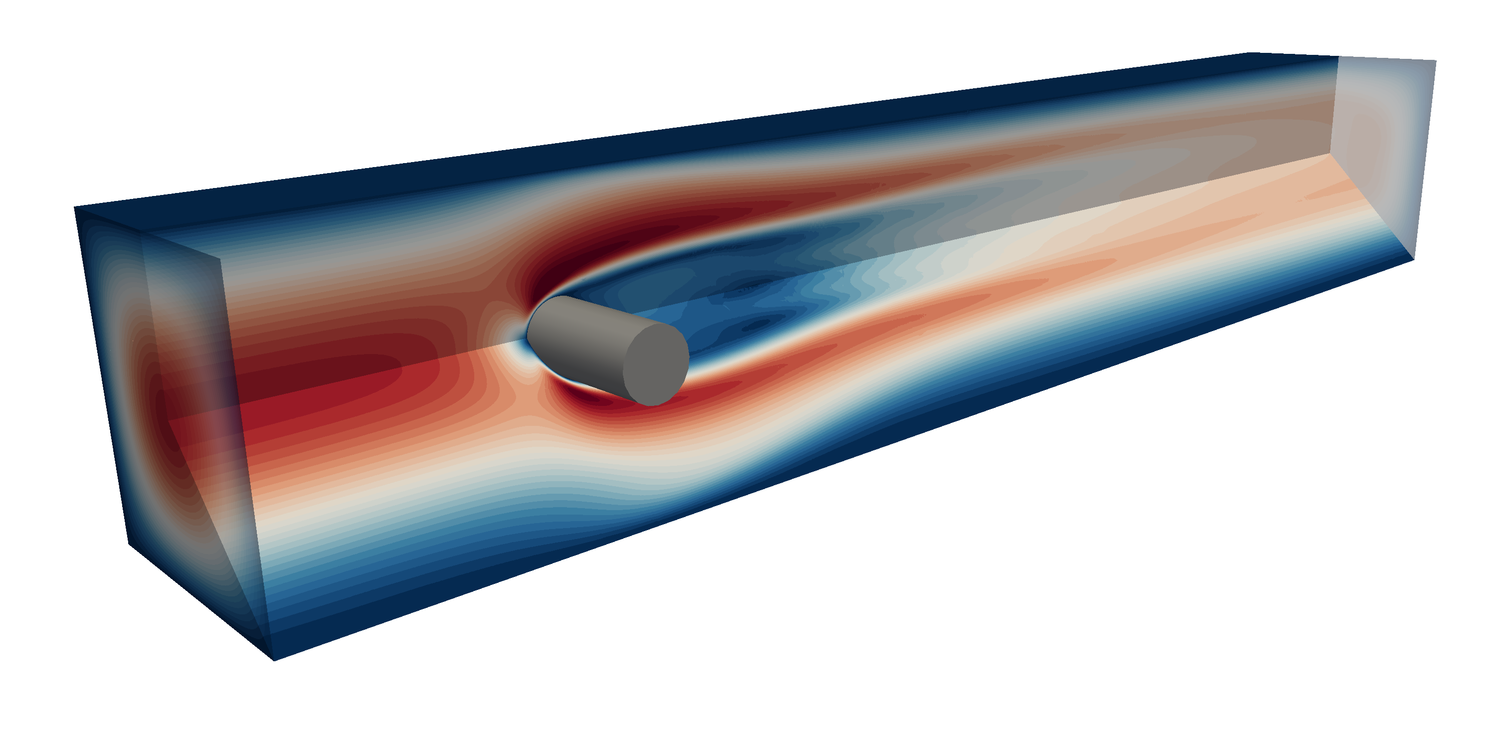
In the Navier-Stokes equations the Reynolds number \(Re\) prescribes the ratio between advective and diffusive forces. If \(Re\) is large -- which is the most important scenario in this project -- boundary layers form at the wall boundary. To capture the macroscopic flow behavior these boundary typically need to be resolved, i.e. the computational mesh needs to be sufficiently fine to be able to represent the flow profile accurately. Ideally, if the boundary layer behavior would be known by proper modeling, the macroscopic flow behavior could also be captured by incorporating the boundary layer profile in the modeling, e.g. by the application of adjusted boundary conditions.

Project goal and further details

In this project a feature map that takes local macroscopic flow information and returns boundary layer profiles in a suitable parametrization shall be learned with machine learning tools. Incorporating the thusly obtained model into the a flow solver is not part of this project.

The following sections define several milestones of this project. These may need to be adapted during the project. In the final section a more concrete list of tasks and rules is given (though still incomplete and not necessarily presented in the correct order).

1. Setup of simulation environment

In a first step the simulation setup that contain the data that can be used for learning the feature map needs to be set up. This includes the following steps:

• Installation of Netgen/NGSolve [1,2]
• Running a simple Navier Stokes discretization as in py_tutorials/navierstokes.py or the i-tutorials of NGSolve [2]Running these examples should initially only check if the installation setup is working properly
• Installation of NGSolve model templates and test run of Navier-Stokes example [2]Again, running these examples should initially only check if the installation setup is working properly. Afterwards it is a good candidate for the black box flow solver that can be used
• Setup a git repository (gitlab.gwdg.de) for the project

2. Setup of flow configurations

In this step several flow configuration with

• varying Reynolds numbers and
• varying geometries shall be setup. Furthermore several wall boundary locations and time points shall be gathered that can later on serve as the points from where the data for the learning can be extracted. Think a proper format to store these points (and normal directions).

3. Definition of the feature map

Think about a list of quantities for a suitable feature map (for the collection of data the list of features may be larger then what you use later on). Possibilities:

Possible input features:

• pressure gradient
• tangential comp. of pressure gradient
• vorticity
• viscosity
• velocity (at some distance to the boundary)
• tangential velocity (at some distance to the boundary)
• ...

Possible output features:

• Cubic spline control points for the graphs of the
  • tangential velocity over wall distance
  • pressure over wall distance
• ...

4. Evaluation of features from flow solution

Write a method that evaluate for a given discrete flow field the input and output features based on point evaluations and averages.

5. Examplary collection of data

Make a dry-run and collect from a subset of all points some data necessary to learn the feature map.

6. Training a neural net

Define a suitable neural net. Pick a suitable library (pytorch, tensorflow) to set up a suitable neural net and feed it with the example data from 5.

7. Evaluate and improve neural net

Now, train the neural net with a significant amount of data and evaluate the prediction based on:

1. data points that are part of the training set
2. data points that are beyond the training set Also experiment around with data points that have are far away (e.g. when \(Re < 100\) has been used for training, try \(Re > 1000\), etc..)

The results may also depend on the selection of the features in the feature map. Also "play around" with these. Try to find a suitable (most robust) set of features.

A list of tasks and rules

Format of the project result

The project shall result in a git-repository containing the following:

• the source code (python),
• API documentation for the code (pydoc/sphinx),
• further documentation on the methods (markdown, gitlab pages, html, latex,..)
• continuous integration facilities including an automatic evaluation of a (gitlab CI / github actions)
• test suite (pytest, ...) As such the repository replace the submission of a usual report. Make sure that you include usable and understandable examples in the repo (i.e. your submission).

Some guidelines

Here are some suggested guidelines

• most of the stuff that you have to learn during the project should be documented. The result should be accessible for students that are in the state of knowledge that you had when you started the project.
• use gitlab issues to set up ToDo-items and organize assignments, etc..
• git: prefer many small commits over few large commits
• use branches and merge (requests) when working on the repo in parallel
• document the structure and the file organization in text-based files (e.g. markdown) in the repository
• for every new feature that you use, set up a test case with automated testing in the gitlab CI
• In a top-level file - similar to this description - write down the project goal an the steps achieved (where/how)
• Interactive demos such as jupyter notebooks are welcome and can serve as part of an "extended documentation"
• Write a log to keep track of the "history" of the project so that you can still explain and understand how the project developed the way it did.

References

[1] J. Schöberl et al., NGSolve software homepage

[2] J. Schöberl et al., NGSolve installation instructions